Peak Fitting

The analysis.peak_fitting module performs non-linear least-squares deconvolution of XPS peaks using Voigt, Gaussian, and Lorentzian lineshape models.

Lineshape Models

Gaussian

Instrumental broadening is modeled as a Gaussian:

\[ G(E; A, \mu, \sigma) = \frac{A}{\sigma \sqrt{2\pi}} \exp\left[-\frac{(E - \mu)^2}{2\sigma^2}\right] \]

Lorentzian

Core-hole lifetime broadening follows a Lorentzian:

\[ L(E; A, \mu, \gamma) = \frac{A}{\pi} \cdot \frac{\gamma}{(E - \mu)^2 + \gamma^2} \]

Voigt

The Voigt profile convolves Gaussian and Lorentzian broadening. Computed via the Faddeeva function \(w(z)\):

\[ V(E; A, \mu, \sigma, \gamma) = A \cdot \frac{\text{Re}[w(z)]}{\sigma \sqrt{2\pi}} \]

where \(z = (E - \mu + i\gamma) / (\sigma \sqrt{2})\).

from xps_analyzer.analysis import fit_voigt, fit_gaussian, fit_lorentzian

# Voigt profile (most physically accurate for XPS)
result = fit_voigt(spectrum, position=284.8, fwhm=1.2)

# Access results
print(f"Position: {result.peaks[0].position:.2f} eV")
print(f"FWHM: {result.peaks[0].fwhm:.2f} eV")
print(f"R²: {result.r_squared:.4f}")

Multi-Peak Deconvolution

For complex envelopes with overlapping components:

from xps_analyzer.analysis import fit_multiple_peaks

result = fit_multiple_peaks(
    spectrum,
    positions=[284.8, 286.2, 287.5, 289.0],
    models=["voigt", "voigt", "voigt", "voigt"]
)

Spin-Orbit Doublets

Spin-orbit coupling produces characteristic doublet peaks with fixed energy separation and area ratio:

\[ \text{Area ratio} = \frac{2j_{\text{high}} + 1}{2j_{\text{low}} + 1} \]

Orbital	\(j\) values	Separation	Area Ratio
p (\(l=1\))	1/2, 3/2	Variable	1:2
d (\(l=2\))	3/2, 5/2	Variable	2:3
f (\(l=3\))	5/2, 7/2	Variable	3:4

from xps_analyzer.analysis import fit_doublet

# Ti 2p doublet
result = fit_doublet(
    spectrum,
    peak_position=458.7,       # Ti 2p_3/2 position
    separation=5.7,             # Spin-orbit splitting
    area_ratio=0.5              # p-orbital branching ratio
)

Physical Constraints

The doublet fitting enforces:

Fixed energy separation between components
Constrained area ratio within configurable tolerance
Equal FWHM for both components
Shared background parameters

Optimization

All fitting uses Levenberg-Marquardt (via lmfit) with:

\(\chi^2\) minimization objective
Analytical Jacobians for Gaussian/Lorentzian
Bounds on FWHM (\(> 0\)), position (\(\pm\) 5 eV window), and amplitude
Convergence tolerance: \(\Delta\chi^2 < 10^{-6}\)

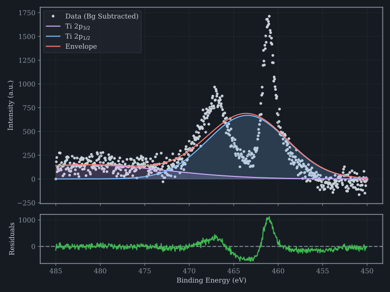Peak fitting example Voigt doublet deconvolution of a Ti 2p spectrum. The lower panel shows the residual.